Magnetic Resonance Fingerprinting (MRF) [Ma2013] is a quantitative technique with potential to improve the feasibility of quantitative MRI measurements in clinical environments.
This post describes the principles of MRF and introduces some of the published research that has been conducted to improve aspects of it. The content of this post is largely based on [Allen2019].
Original Framework
MRF was developed to simultaneously measure multiple MR properties, such as T1 and T2, using a single acquisition. The method allows short scan durations, with the original MRF publication showing improved time efficiency compared with two single-parameter sequences (DESPOT1 and DESPOT2) [Ma2013].
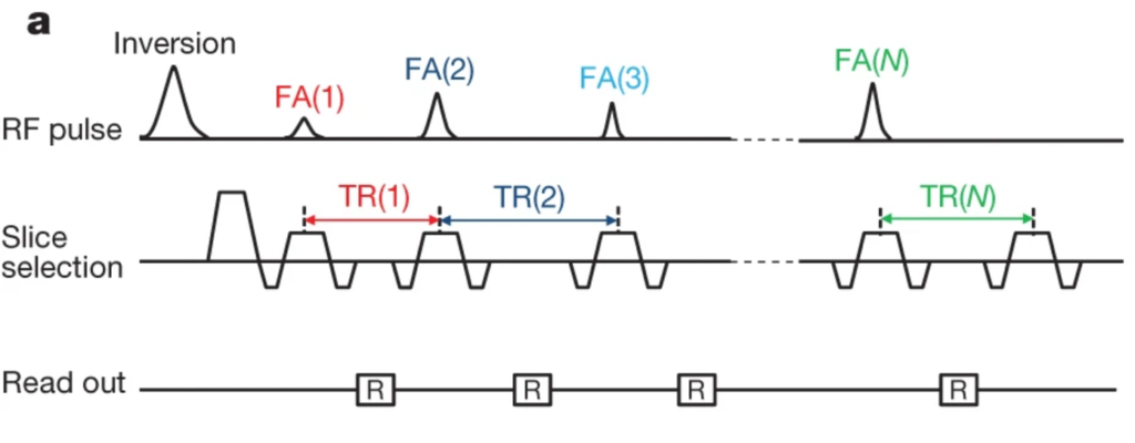
During an MRF experiment, a sequence with a pseudo-random set of parameters is used to manipulate spins in a sample and acquire images. In the ideal case, each tissue type within a sample produces a unique signal timecourse through the set of images. This can be achieved by varying the time between subsequent RF pulses and the size of any RF-induced magnetisation rotations (Fig. 1).
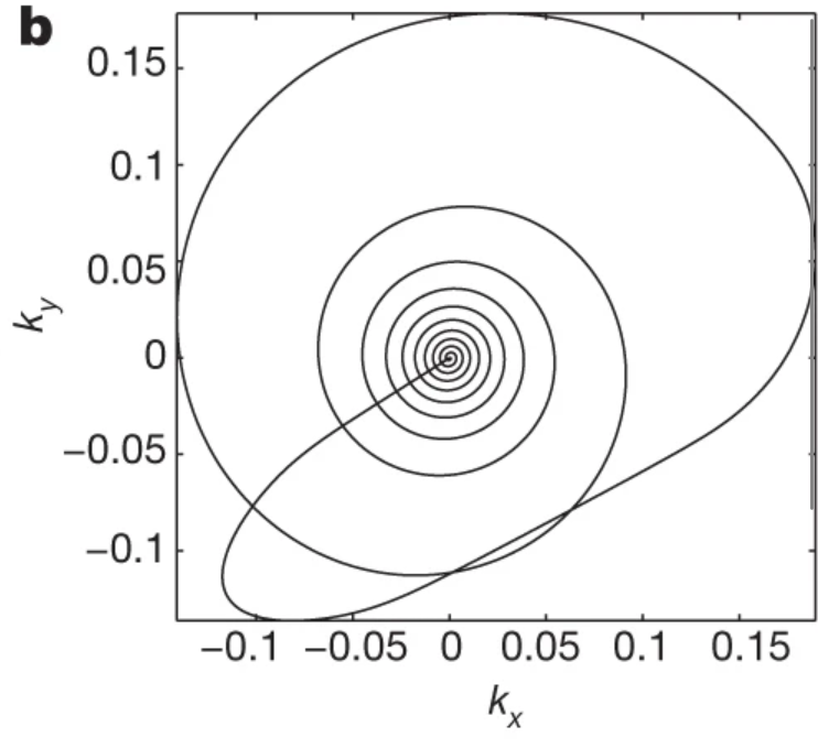
MRF is commonly implemented with interleaved k-space undersampling to achieve fast data acquisition, where the k-space trajectory is rotated between each image acquisition to produce some incoherence between the underlying signal and the image artefacts (Fig. 2).
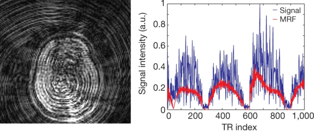
For a given pixel, the signal timeseries over the whole experiment is compared to a previously built dictionary of simulated signal patterns to find the closest match (Fig. 3). The dictionary is compiled by simulating the signal expected from the particular acquisition parameters and sequence structure for all combinations of the chosen tissue and system parameters (e.g. T1 and T2) over given ranges.
Finally, the tissue parameters used to simulate the best-matched dictionary timecourse are assigned to the pixel. This process is repeated for every pixel.
Subsequent Developments
The original MRF proof-of-principle [Ma2013] was based on a balanced SSFP (bSSFP) sequence with an initial inversion pulse (Fig. 1), producing maps of T1, T2, modulated M0, and B0 inhomogeneity in an acquisition time of approximately 12 seconds per slice. TR and FA were varied. Each TE was set as half of the corresponding TR, as is typical for bSSFP acquisitions.
Subsequent developments have been made regarding the sequence design, image reconstruction, and parameter assignment.
FISP MRF
An unbalanced version of the original bSSFP sequence (i.e. SSFP), has become widely used for MRF due to its inherent insensitivity to B0 inhomogeneity [Jiang2014, Asslander2017]. The SSFP sequence is usually known as FISP. Subsequent versions have extended FISP MRF to a 3D acquisition, giving whole brain T1, T2 and modulated M0 maps in less than 5 minutes [Ma2017]. In the original implementation of FISP MRF TE was fixed throughout the acquisition [Jiang2014] but the FA schedule pattern was smoother than that used in the original bSSFP MRF paper [Ma2013].
Additional Parameter Maps
Alterations to the original MRF framework have enabled other tissue properties and system characteristics to be measured.
Additional preparation pulses have been used to evoke sensitivity to diffusion [Christen2014, Rieger2018] and perfusion [Su2017].
Christen et al. [Christen2014] used a cerebral vascular model to estimate maps of cerebral blood volume, mean vessel radius and blood oxygen saturation. In [Christen2014] a hybrid gradient-echo and spin-echo sequence was used to sample gradient echoes before and after the spin echo, as well as the spin echo signal itself. Signal evolution curves were acquired with and without a contrast agent, with the ratio of the two curves used as a fingerprint.
Anderson et al. [Anderson2017] detected and quantified concentrations of multiple contrast agents after simultaneous administration.
Hong et al. [Hong2019] simultaneously estimated T1 , T2 , T2∗, M0 and B0 using a hybrid of FISP and spoiled gradient-echo squences.
The partial volume effect can also be accounted for and mapped [Deshmane2014, Tang2018, McGivney2019].
The spatial variation of the radiofrequency (RF) excitation field B1+ can be mapped by including an extra dimension in the dictionary. This approach requires that the effects of T1 and B1+ variations can be distinguished. One way of ensuring this is to design the RF flip angle schedule [Buonincontri2016, Buonincontri2017] such that the dictionary fingerprints vary differently as a function of B1+ and T1. An alternative to accounting for B1+ variations in the dictionary is to use an externally-acquired reference B1+ efficiency map to scale the flip angles during the production of the dictionary, generating a tailored dictionary for each pixel [Ma2017].
Dictionary Simulation
When a dictionary is used to produce MRF parameter maps each fingerprint is assigned to one of the dictionary entries. This means the sizes of the dictionary dimension increments affect the accuracy and precision of the resulting parameter maps. For example, large steps in T1 could worsen the parameter map accuracy if the true T1 values are between the dictionary T1 values.
The incorporation of slice profile simulations during the dictionary generation has been shown to improve parameter assignment accuracy [Hong2017, Chiu2017] for flip angle regimes often used in MRF sequences.
Reductions in dictionary dimensionality [McGivney2014] and clustering [Cauley2015] have enabled more efficient dictionary searching, decreasing the computational cost of the matching process. One of the examples in [McGivney2014] was the temporal compression of a bSSFP MRF dictionary with 363624 entries and 1000 timepoints. When 200 singular values were used to construct this compressed dictionary the matching time (using phantom data) reduced from 31 seconds to 7.3 seconds and there were only 5 pixels with T1 or T2 values that did not exactly match those obtained using the uncompressed dictionary. Each of these differences for those pixels was one step in the corresponding dictionary parameter resolution, highlighting the impact of the dictionary step size on the matching error.
Image Acquisition
Simultaneous multislice acquisitions have been used to further reduce the acquisition time per slice [Ye2016, Ye2017] and alternative sampling strategies have been explored, such as radial [Cloos2016] and Cartesian trajectories. Examples of Cartesian sampling in MRF have included the acquisition of single phase-encoding lines [Gao2015, Anderson2018] and a fully sampled EPI readout [Rieger2017, Rieger2018] per TR. The sequence in [Rieger2018] used pairs of refocusing pulses, allowing sensitivity to T2. Acquiring a fully sampled image for each timepoint reduces the image artefacts and requires comparatively straightforward image reconstruction.
Parameter Map Reconstruction
Reconstruction algorithms and data models have been used to produce parameter maps from the k-space data, with improved parameter accuracy [Zhao2016, Wang2016, Pierre2016]. Amthor et al. [Amthor2015] applied a machine learning algorithm to the MRF matching process to provide tissue parameter maps. Various algorithms were compared for their performance in classifying fingerprints from a bSSFP MRF sequence, with an acquisition made substantially longer because of Cartesian sampling. The data were classified into clusters of T1 and T2 combinations with no exact assignment of B0. Deep learning [LeCun2015] has also been used to provide parameter estimates [Cohen2017, Hoppe2017].
Acquisition Parameter Schedule Optimisation
Cohen et al. [Cohen2017] optimised the acquisition parameter schedule of a gradient-echo EPI sequence by minimising the dot products between the dictionary entries. In [Cohen2017] a collection of algorithms was used to optimise MRF sequences with respect to the global dictionary dot product. An interior-point algorithm was shown to outperform others in terms of the final cost function minimum, the required function iterations and the scan duration of the optimised schedule. In simulations the represented algorithms provided relatively large T2 percentage errors compared to T1. However, the interior-point optimisation provided substantial improvements in T2 compared to the other algorithms. MRF experiment simulations have also been used to estimate the parameter assignment error at each optimisation iteration and aim for a schedule that minimises this error, such as the work by Hamilton et al. [Hamilton2015] which used a genetic algorithm to optimise a FISP MRF schedule. Other work has used Monte Carlo simulations to assess the suitability of a given schedule [Sommer2017].
Signal Modelling
This section includes points to consider when modelling the MRF signal, including comments on the signal modelling approach used for FISP MRF and a discussion on excitation slice profiles.
Extended Phase Graphs
Solutions to the Bloch equations are used to model the behaviour of isochromats and simulate the signals of bSSFP MRF experiments, using a series of matrix rotations and exponential relaxation terms.
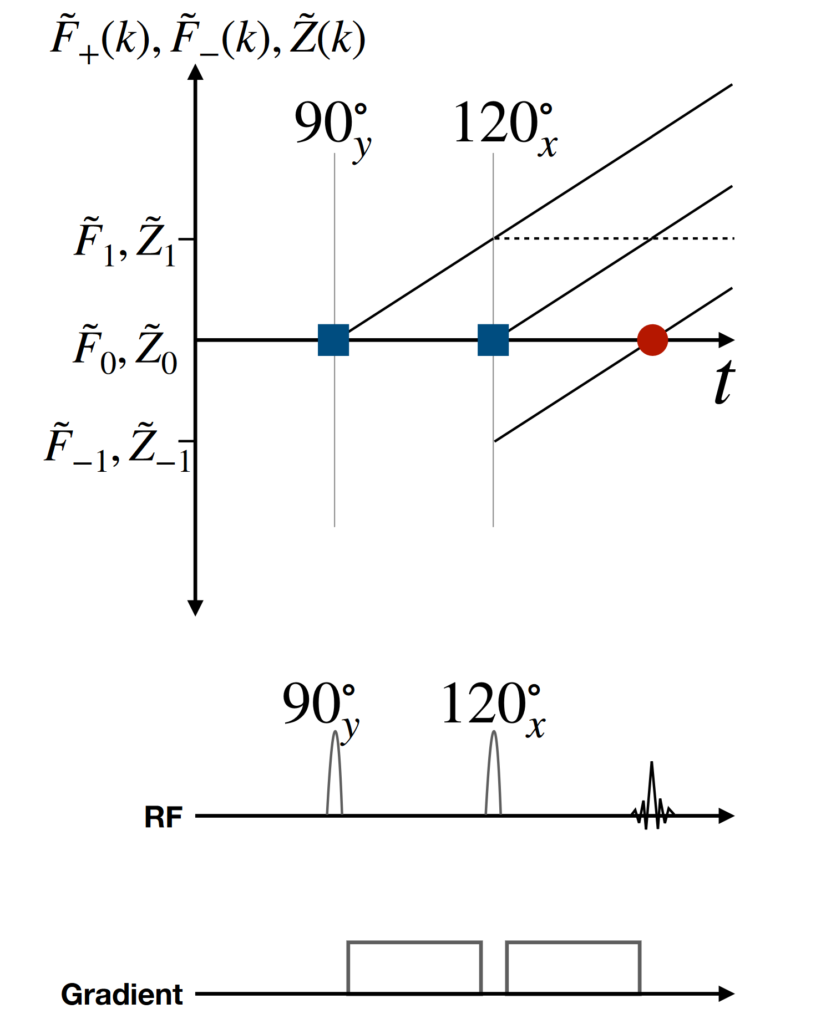
In FISP experiments the dephasing during each TR is not refocused and the acquired signal of each voxel is an average of all the spins inside it. The isochromat model used in bSSFP simulations is not practical for this application because the signal from a large number of isochromats would need to be simulated. The Extended Phase Graph (EPG) formalism is a practical way of modelling signal evolutions throughout unbalanced sequences such as FISP MRF [Jiang2014], simulating the magnitude and temporal positioning of refocused signal echoes.
The EPG formalism can model the effect of RF pulses and gradients on the magnetisation by considering intra-voxel phase distributions in terms of Fourier states, often in units of 2π. Figure 4 shows an example EPG diagram for a simple pulse sequence, with phase states on the y-axis and time on the x-axis. In Fig. 4 the second RF pulse refocuses a component of the magnetisation dephased by the first pulse, causing a signal echo. The rate of transition between states depends on the gradient amplitude. The effects of transverse and longitudinal relaxation on the magnitude of the signal echoes can also be modelled. More details about the principles behind extended phase graphs can be found in [Weigel2015].
Excitation Slice Profiles
Pulse and Gradient Shapes
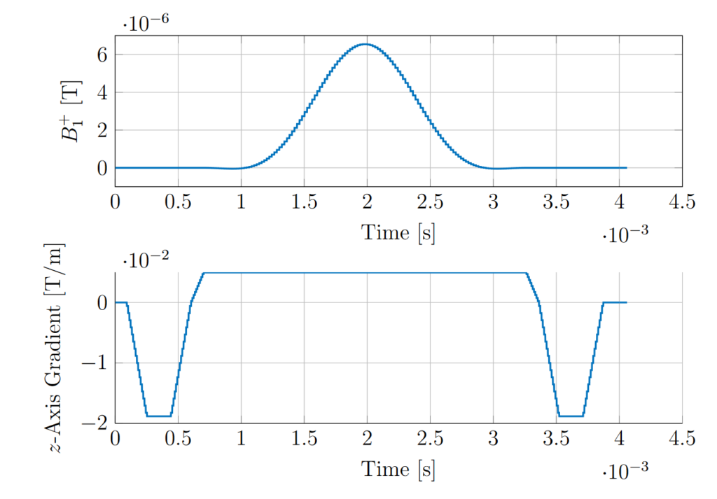
An example slice-selective RF sinc pulse and the corresponding gradient from a balanced SSFP sequence is shown in Fig. 5. The RF pulse has the amplitude required to deliver a 90-degree rotation angle at the slice centre and the gradient has the amplitude required to excite a slice 5mm thick (full width half maximum). The gradient applied during the RF pulse has the effect of dephasing the transverse magnetisation across the slice, meaning the phase of the transverse magnetisation depends on the position along the slice direction. The purpose of the gradient lobe after the RF pulse is to refocus this dephasing. The pre-dephaser lobe before the pulse is specific to balanced SSFP and is not present in FISP and spin-echo pulse sequences.
Non-Ideal Excitation Profile
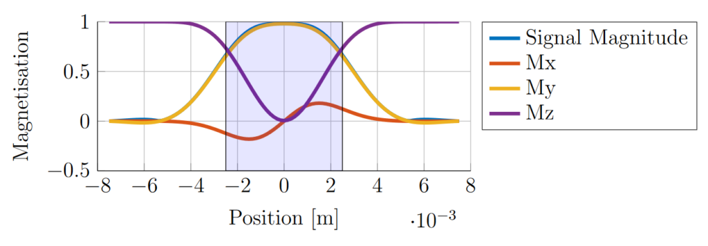
The effect of the RF pulse is to rotate the magnetisation into the transverse plane to produce signal. Ideally, and assuming zero transverse components before the pulse, the signal outside the slice after the slice-selective pulse will remain zero and the spins at all positions through the slice direction will be identically manipulated, producing a top-hat signal magnitude profile through the slice. In practice there is a gradual change in the signal magnitude across the slice edges (Fig. 6). Since the acquired signal is the signal integral across the slice the signal acquired in practice is lower than in the ideal case.
Slice Profile Simulation
For small flip angles, the relationship between the flip angle and the RF field is approximately linear, meaning the slice profile can be estimated by the Fourier transform of the RF pulse shape. For off-resonance pulses or high flip angles the relationship becomes non-linear and numerical simulations are required to determine the slice profile [Bernstein2004]. The numerically-simulated magnetisation profile resulting from the RF sinc pulse and gradient profiles from Fig. 5 is shown in Fig. 6. The pulse profile resembles a Gaussian shape because of the time-bandwidth product of the pulse. The profile of a sinc pulse with a higher bandwidth product would have visible lobes either side of the main peak. The magnetisation at a given position in the slice was a result of the net rotation at that point, which was calculated by simulating the effect of the RF pulse profile at discrete timepoints.
Limitations
When choosing an image acquisition method for MRF it is important to consider the trade-off between the image quality and the number of images required. The majority of MRF methods use undersampled image acquisitions, allowing a large number of measurements in a reasonable timeframe. For example, the interleaved undersampling trajectory in [Ma2013] required between approximately 11ms to 13.5ms per timepoint, although this did mean that the images contained severe undersampling artefacts. Despite the time-varying nature of the artefacts (due to a rotation of the trajectory between timepoints) the signal fluctuations caused by the artefacts meant large numbers of timepoints (e.g. 1000) were required to obtain good fits. Fully sampled EPI images contain less severe artefacts and so can effectively provide a larger SNR. This means that although fully sampled EPI MRF sequences take longer to acquire each timepoint the overall scan duration will not necessarily be extended because fewer timepoints are needed.
Further advances may be made by increasing the signal-to-noise ratio at each acquired timepoint, inducing sensitivity to additional tissue parameters, or improving the acquisition accuracy and temporal efficiency. There may be some overlap between these topics. For example, increasing the signal-to-noise ratio may improve the acquisition accuracy.
Key areas of research are the choice of the base sequence design and optimising the sequence acquisition schedule, including the choice of algorithm and cost function.
References
- J. Allen, ‘An Optimisation Framework for Magnetic Resonance Fingerprinting’. PhD thesis. University of Oxford. 2019. https://ora.ox.ac.uk/objects/uuid:14c92874-7b00-4f79-abce-87b05f9cb4d4
- D. Ma, V. Gulani, N. Seiberlich, K. Liu, J. L. Sunshine, J. L. Duerk, and M. A Griswold. Magnetic resonance fingerprinting. Nature, 495(7440):18792, 2013.
- Y. Jiang, D. Ma, N. Seiberlich, V. Gulani, and M. A. Griswold. MR fingerprinting using fast imaging with steady state precession (FISP) with spiral readout. Magnetic Resonance in Medicine, 74(6):1621–1631, 2014.
- J. Asslander, S. J. Glaser, and J. Hennig. Pseudo Steady-State Free Precession for MR-Fingerprinting. Magnetic Resonance in Medicine, 77(3):11511161, 2017.
- D. Ma, S. Coppo, Y. Chen, D. F. McGivney, Y. Jiang, S. Pahwa, V. Gulani, and M. A. Griswold. Slice profile and B1 corrections in 2D magnetic resonance fingerprinting. Magnetic Resonance in Medicine, 78(5):1781–1789, 2017.
- T. Christen, N. A. Pannetier, W. W. Ni, D. Qiu, M. E. Moseley, N. Schuff, and G. Zaharchuk. MR vascular fingerprinting: A new approach to compute cerebral blood volume, mean vessel radius, and oxygenation maps in the human brain. NeuroImage, 89:262–270, 2014.
- B. Rieger, M. Akcakaya, L. R. Schad, and S. Weingartner. Simultaneous quantification of T1, T2 and Apparent Diffusion Coefficient using Magnetic Resonance Fingerprinting based on Echo Planar Imaging. In Proceedings of the 26th Annual Meeting of ISMRM, page 1023, 2018.
- P. Su, D. Mao, P. Liu, Y. Li, M. C. Pinho, B. G. Welch, and H. Lu. Multiparametric estimation of brain hemodynamics with MR fingerprinting ASL. Magnetic Resonance in Medicine, 78(5):1812–1823, 2017.
- C. E. Anderson, S. B. Donnola, Y. Jiang, J. Batesole, R. Darrah, M. L. Drumm, S. M. Brady-Kalnay, N. F. Steinmetz, X. Yu, M. A. Griswold, and C. A. Flask. Dual Contrast – Magnetic Resonance Fingerprinting (DCMRF): A Platform for Simultaneous Quantification of Multiple MRI Contrast Agents. Scientific Reports, 7(1):8431, 2017.
- T. Hong, D. Han, and D-H. Kim. Simultaneous estimation of PD, T1, T2, T2*, and B0 using magnetic resonance fingerprinting with background gradient compensation. Magnetic Resonance in Medicine, 81(4):2614–2623, 2019.
- A. Deshmane, D. Ma, Y. Jiang, E. Fisher, N. Seiberlich, V. Gulani, and M. Griswold. Validation of Tissue Characterization in Mixed Voxels Using MR Fingerprinting. In Proceedings of the 22nd Annual Meeting of ISMRM, page 94, 2014.
- S. Tang, C. Fernandez-Granda, S. Lannuzel, B. Bernstein, R. Lattanzi, M. Cloos, F. Knoll, and J. Asslander. Multicompartment Magnetic Resonance Fingerprinting. Inverse Problems, 34(9):094005, 2018.
- D. F. McGivney, D. Ma, Y. Jiang, A. Deshmane, V. Gulani, N. Seiberlich, and M. A. Griswold. Partial volume mapping using magnetic resonance fingerprinting. NMR in Biomedicine, 32(5):e4082, 2019.
- G. Buonincontri and S. J. Sawiak. MR fingerprinting with simultaneous B1 estimation. Magnetic Resonance in Medicine, 76(4):1127–35, 2016.
- G. Buonincontri, R. F. Schulte, M. Cosottini, and M. Tosetti. Spiral MR fingerprinting at 7 T with simultaneous B1 estimation. Magnetic Resonance Imaging, 41:1–6, 2017.
- T. Hong, D. Han, M-O. Kim, and D-H. Kim. RF slice profile effects in magnetic resonance fingerprinting. Magnetic Resonance Imaging, 41:73–79, 2017.
- S-C. Chiu, T-M. Lin, J-M. Lin, H-W. Chung, C-W. Ko, M. B ̈ uchert, and M. Bock. Effects of RF pulse profile and intra-voxel phase dispersion on MR fingerprinting with balanced SSFP readout. Magnetic Resonance Imaging, 41:80–86, 2017.
- D. F. McGivney, E. Pierre, D. Ma, Y. Jiang, H. Saybasili, V. Gulani, and M. A. Griswold. SVD compression for magnetic resonance fingerprinting in the time domain. IEEE Transactions on Medical Imaging, 33(12):2311–2322, 2014.
- S. F. Cauley, K. Setsompop, D. Ma, Y. Jiang, H. Ye, E. Adalsteinsson, M. A. Griswold, and L. L. Wald. Fast group matching for MR fingerprinting reconstruction. Magnetic Resonance in Medicine, 74(2):523–528, 2015.
- H. Ye, D. Ma, Y. Jiang, S. F. Cauley, Y. Du, L. L. Wald, M. A. Griswold, and K. Setsompop. Accelerating magnetic resonance fingerprinting (MRF) using t-blipped simultaneous multislice (SMS) acquisition. Magnetic Resonance in Medicine, 75(5):2078–85, 2016.
- H. Ye, S. F. Cauley, B. Gagoski, B. Bilgic, D. Ma, Y. Jiang, Y. P. Du, M. A. Griswold, L. L. Wald, and K. Setsompop. Simultaneous multislice magnetic resonance fingerprinting (SMS-MRF) with direct-spiral slice-GRAPPA (dsSG) reconstruction. Magnetic Resonance in Medicine, 77(5):1966–1974, 2017.
- M. A. Cloos, F. Knoll, T. Zhao, K. Block, M. Bruno, C. G. Wiggins, and D. K. Sodickson. Multiparametric imaging with heterogenous radiofrequency fields. Nature Communication, 7:12445, 2016.
- Y. Gao, Y. Chen, D. Ma, Y. Jiang, K. A. Herrmann, J. A. Vincent, K. M. Dell, M. L. Drumm, S. M. Brady-Kalnay, M. A. Griswold, C. A. Flask, and L. Lu. Preclinical MR fingerprinting (MRF) at 7 T: Effective quantitative imaging for rodent disease models. NMR in Biomedicine, 28(3):384–394, 2015.
- C. E. Anderson, C. Y. Wang, Y. Gu, R. Darrah, M. A. Griswold, X. Yu, and C. A. Flask. Regularly incremented phase encoding – MR fingerprinting (RIPE-MRF) for enhanced motion artifact suppression in preclinical cartesian MR fingerprinting. Magnetic Resonance in Medicine, 79(4):2176–2182, 2018.
- B. Rieger, F. Zimmer, J. Zapp, S. Weing ̈ artner, and L. R. Schad. Magnetic resonance fingerprinting using echo-planar imaging: Joint quantification of T1 and T2* relaxation times. Magnetic Resonance in Medicine, 78(5):17241733, 2017.
- B. Zhao, K. Setsompop, H. Ye, S. Cauley, and L. L Wald. Maximum Likelihood Reconstruction for Magnetic Resonance Fingerprinting. IEEE Trans Med Imaging, 35(8):1812–23, 2016.
- Z. Wang, H. Li, Q. Zhang, J. Yuan, and X. Wang. Magnetic Resonance Fingerprinting with compressed sensing and distance metric learning. Neurocomputing, 174:560–570, 2016.
- E. Y. Pierre, D. Ma, Y. Chen, C. Badve, and M. A. Griswold. Multiscale reconstruction for MR fingerprinting. Magnetic Resonance in Medicine, 75(6):2481–2492, 2016.
- T. Amthor, M. Doneva, P. Koken, J. Keupp, and P. Bornert. Comparison of Different Approaches of Pattern Matching for MR Fingerprinting. In Proceedings of the 23rd Annual Meeting of ISMRM, page 3394, 2015.
- Y. LeCun, Y. Bengio, and G. Hinton. Deep learning. Nature, 521(7553):436, 2015.
- O. Cohen, B. Zhu, and M. S. Rosen. Deep learning for fast MR Fingerprinting Reconstruction. In International Society for Magnetic Resonance in Medicine (ISMRM), page 688, 2017.
- E. Hoppe, G. Korzdorfer, T. Wurfl, J. Wetzl, F. Lugauer, J. Pfeuffer, and A. Maier. Deep learning for magnetic resonance fingerprinting: A new approach for predicting quantitative parameter values from time series. GMDS, pages 202–206, 2017.
- O. Cohen and M. S. Rosen. Algorithm comparison for schedule optimization in MR fingerprinting. Magnetic Resonance Imaging, 41:15–21, 2017.
- J. I. Hamilton, K. L. Wright, Y. Jiang, L. Hernandez-Garcia, D. Ma, M. Griswold, and N. Sieberlich. Pulse sequence optimization for improved MRF scan efficiency. In Proceedings of the 23rd Annual Meeting of ISMRM, volume 23, page 3386, 2015.
- K. Sommer, T. Amthor, M. Doneva, P. Koken, J. Meineke, and P. Bornert. Towards predicting the encoding capability of MR fingerprinting sequences. Magnetic Resonance Imaging, 41:7–14, 2017.
- M. Weigel. Extended phase graphs: Dephasing, RF pulses, and echoes – Pure and simple. Journal of Magnetic Resonance Imaging, 41(2):266–295, 2015.
