For my PhD thesis [Allen2019], we produced a custom phantom for evaluating quantitative MRI pulse sequences. We compared fitted Magnetic Resonance Fingerprinting (MRF) parameters with those of reference gold standard sequences. In this post, I’ll share how we implemented a reference T2 method based on the gold standard approach with various echo times. This is related to my introductory post on T2.
For reference T2 estimates, we used a single-echo spin-echo Echo Planar Imaging (EPI) pulse sequence, varying the Echo Time (TE) across the measurements.
Data acquisition
Multiple single-slice images were acquired, each with a different TE, using a Siemens spin-echo EPI sequence. The echo times and repetition times were (min:increment:max) TE = [21:4:69, 80, 90, 110, 200, 400, 800, 1200, 1600, 3200] ms and TR = 30000ms, making the total scan time 660 seconds (i.e. 11 minutes). Other acquisition parameters were: field of view = 250mm × 250mm, in-plane pixel size = 3.9mm × 3.9mm, slice thickness = 5mm, readout bandwidth = 2298Hz per pixel and partial Fourier factor = 6/8.
Model and fitting
To estimate T2, an exponential decay model (Eq. 1) was fitted to the magnitude images. The model included an offset term C to account for positive signal offsets. Although a simple offset correction was used here (Eq. 1) it would be worth considering alternatives in future work, such as squaring the signal [He2008] or removing low SNR data points from the curve [Miller1993].
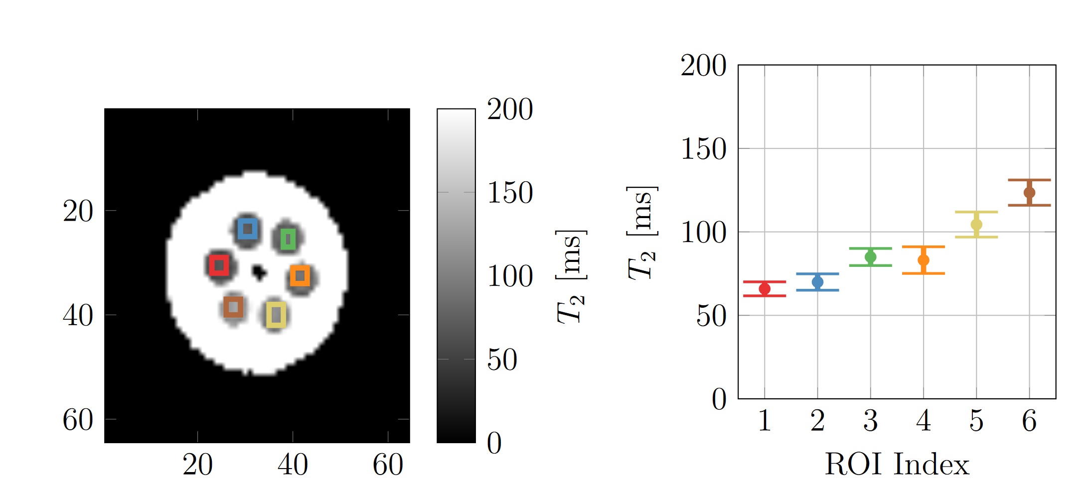
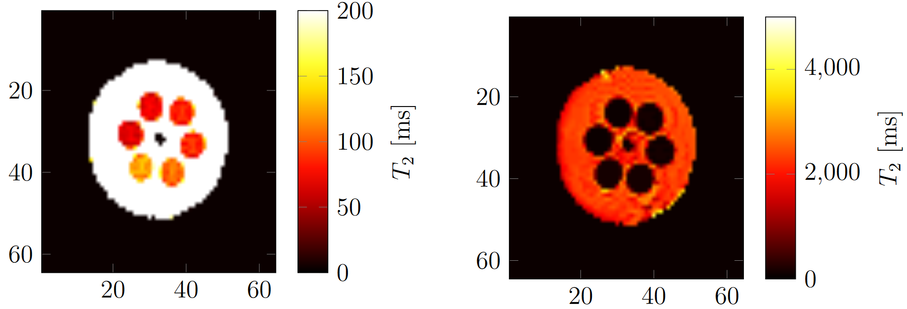
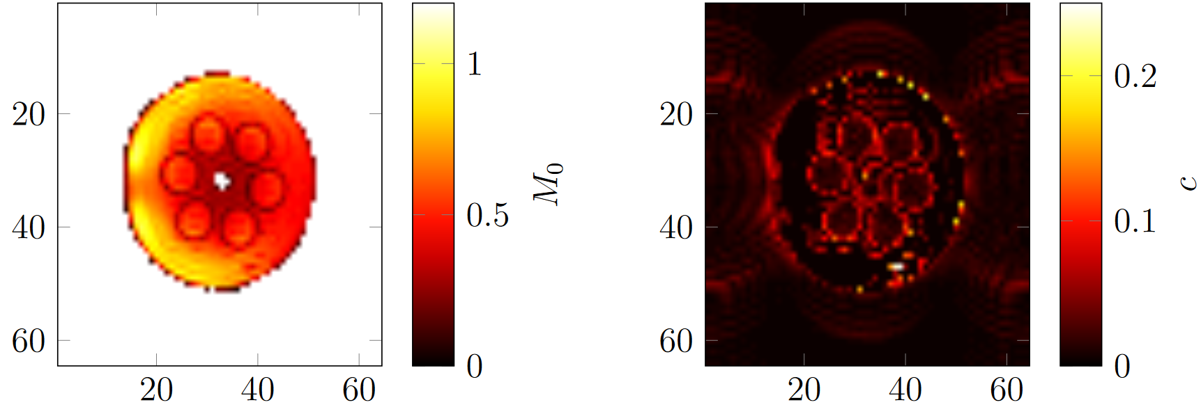
To perform the fit, the MATLAB fit function was used with the default algorithm. Fitted parameter maps of our custom phantom are shown in Fig. 1. Figure 2 shows the T2 distribution across the six inner compartment tubes in the phantom.

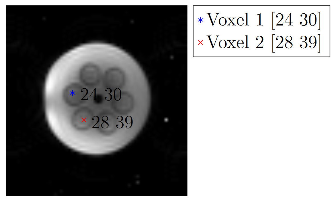
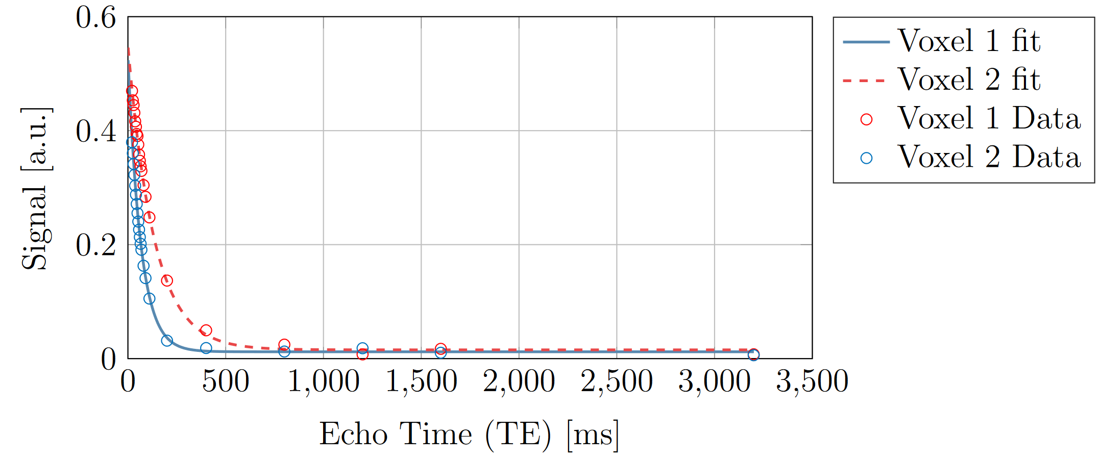
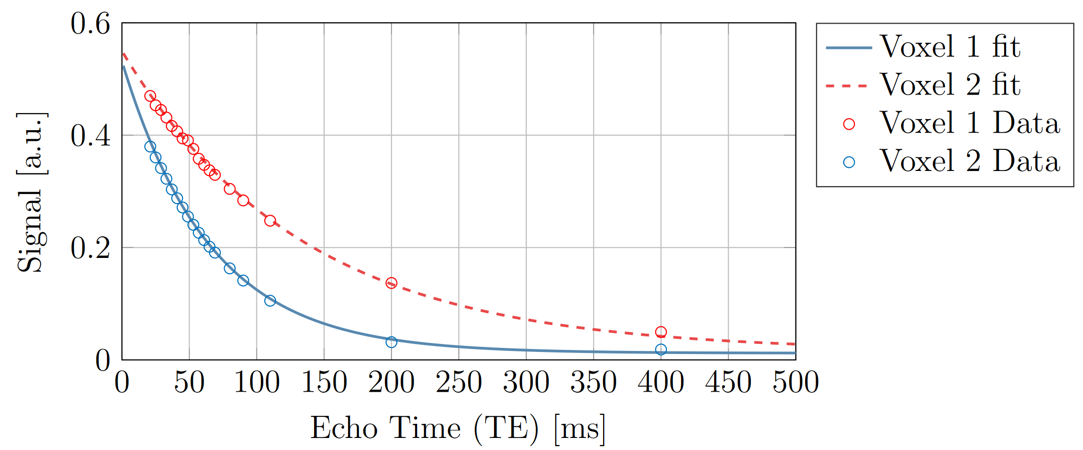
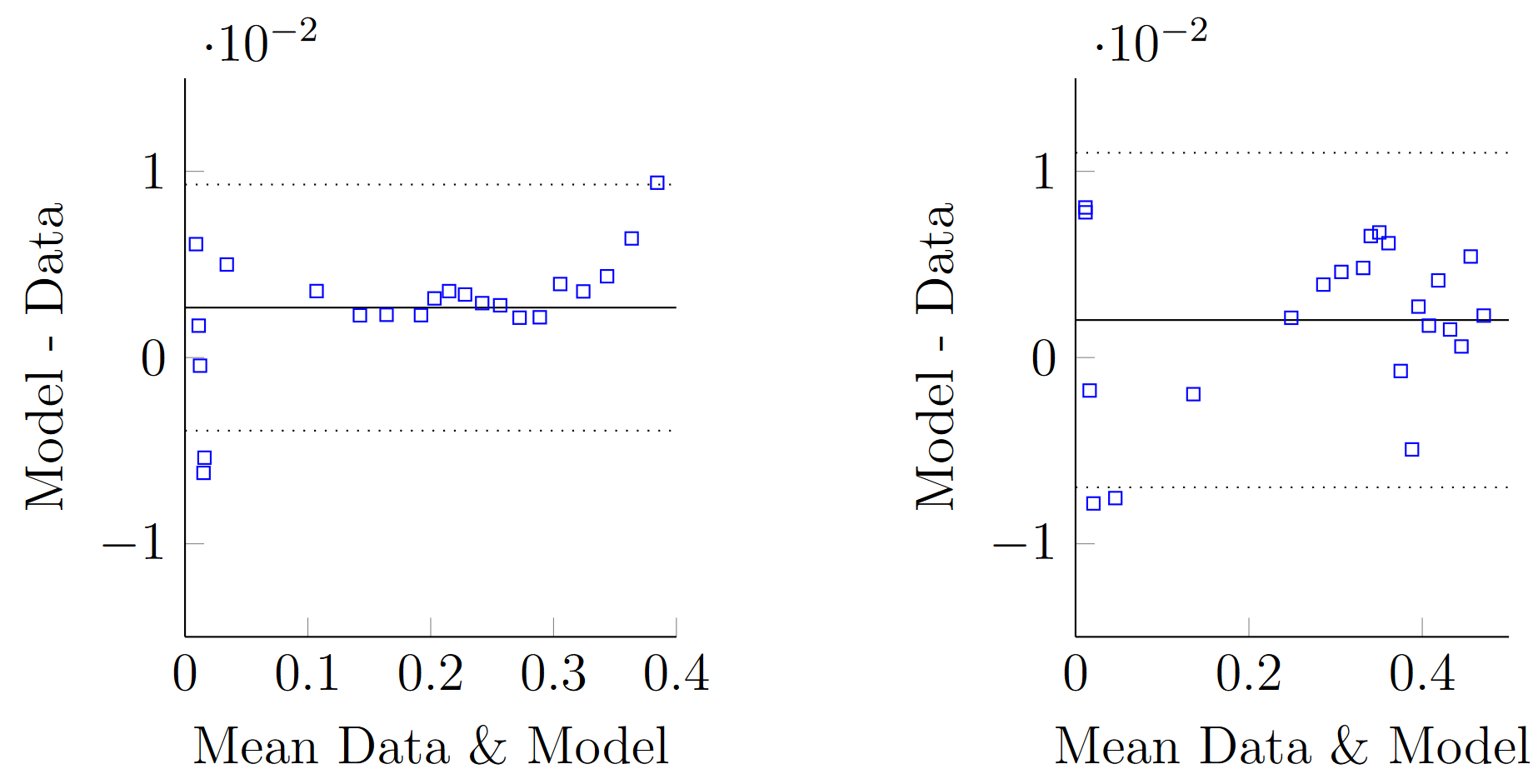
Example fits for voxels from the tubes with the longest and shortest T2 are shown in Fig. 3, with corresponding Bland-Altman plots in Fig. 4. Bland-Altman plots provide a visual representation of measurement bias and confidence. Figure 4 shows the majority of the fitted points were within the 95% confidence interval. However, both plots in Fig. 4 show a positive bias.
Minimum scan time
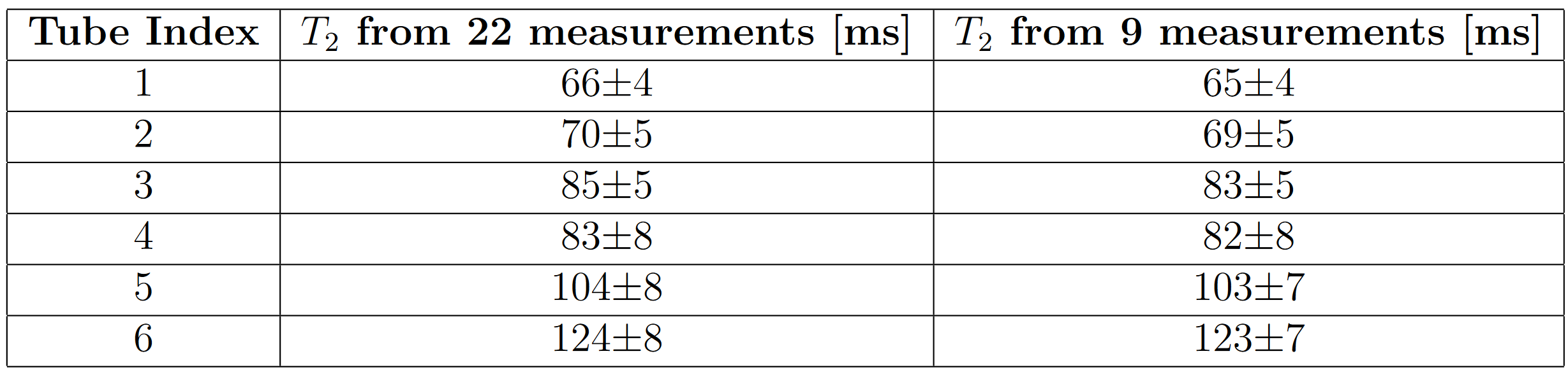
The scan time required by the T2 protocol can be reduced by acquiring fewer measurements. Table 1 compares the tube T2 values obtained from fitting with 22 and 9 measurements from the same data set. The 9 different TEs were [21, 33, 45, 65, 80, 110, 200, 400, 800] ms. Using 9 measurements reduces the scan duration for a single slice to 270 seconds (i.e. 4 minutes 30 seconds), for TR = 30 seconds. The two sets of values in Table 1 are in very close agreement and approximately cover the literature values for grey and white matter [82, 71]. The measured standard deviations in the tubes were between ≈6-10% of the respective means.
The minimum TR for this method can be derived from gold standard T1 measurements of the same phantom. In a separate experiment we measured the longest T1 as 1621ms +/- 23ms. The solution to the longitudinal term of the Bloch equation shows us that for the upper value of this T1 range (i.e. T1 = 1621ms + 23ms), after 10000ms the Mz has effectively recovered. Specifically, 10000ms after a complete inversion Mz will equal 0.995M0, where M0 is the thermal equilibrium value of Mz. By reducing the TR to 10000ms, the scan duration of our reference T2-mapping sequence could be reduced to 90 seconds (i.e. 1 minute 30 seconds) per slice. This would translate to a scan duration of 30 minutes to acquire 20 slices.
References and further reading:
- Allen J. An Optimisation Framework for Magnetic Resonance Fingerprinting. Thesis. University of Oxford, UK. 2019. https://ora.ox.ac.uk/objects/uuid:14c92874-7b00-4f79-abce-87b05f9cb4d4
- T. He, P. D. Gatehouse, G. C. Smith, R. H. Mohiaddin, D. J. Pennell, and D. N. Firmin. Myocardial T2* Measurements in Iron Overloaded Thalassemia: An In Vivo Study to Investigate the Optimal Methods of Quantification. Magnetic Resonance in Medicine, 60(5):1082–1089, 2008.
- A. J Miller and P. M. Joseph. The Use of Power Images to Perform Quantitative Analysis on Low SNR MR Images. Magnetic Resonance Imaging, 11(7):1051–1056, 1993.